Below is a bit of a master doc personally of all my OSPF notes, previously I was keeping this hidden away in a google doc but I thought why not share it with the world. If you see any issues let me know!
These notes are prefect for some general study or some quick interview prep!

But more importantly, if you have any questions or don’t understand something, post a comment and I might be able to help! I always say, the best way to learn something is by teaching it.

1 – Summary

• OSPF is an open standard link state routing protocol which means its accepted by different vendors. 
• An instance of OSPF will know about the whole network/Area and not just routes. It knows about the connections between devices and their associated areas and interfaces.
• Each device will have a full database for its local area which should be identical to others in the area.
• OSPF will always pick the best path from its opinion rather than what a neighbour thinks is best. 
• We have the concept of Areas to reduce the scale of information devices have, being in a non backbone area can reduce the amount of information a device has to process. 
• Routing decisions are based on a number of rules around inter/intra area selection however otherwise in a flat area 0 network the decision is based on a shortest path first decision. 
• The shortest path is determined by a metric based on the bandwidth of links between point A and B. 

2 – Adjacency setup

The 5 high level states of OSPF protocol operation

1 – Establishing adjacencies.

• Down state – nothing has been sent or received and the adjacency hasn’t been initialized
• init state – Indicates a hello has been sent but one hasn’t been received or a hello has been received without the local RID in the list of neighbours or finally that the OSPF hello parameters don’t match
• two way state – Received Hello message with Local RID in the list of neighbours and passing all checks. This identifies that the adjacency is valid and can process further messages

2 – Electing DR and BDR

This is only done in Multi access networks only (i.e 1 node connected to 2 or more nodes through a single interface) This is typically seen on ethernet links unless they are specified as a point to point link

This state isn’t an official state but in this step we decide who is going to be DR and BDR based on ospf priority.
More details to be found in the Multi access networks section.

3 – Discovering routes

• ExStart State – Decides who starts the exchange. (See Primary/Secondary election)
• Exchange state – Sends DBD packets containing LSA headers for all the LSAs in the local LSDB’s
  • See the OSPF messages – DBD section for more
• Loading state – Based on the DBD messages from the previous step the device utilizes:
  • link state request messages to request further details for any LSA it doesn’t currently know about.
  • Requests are followed up by Link state updates containing a number of full LSA’s within it.
  • Finally Link state acknowledgements are sent back to the originating route with full LSA’s again to confirm reception of the new LSA’s 
• Full state – At this state the LSDB’s between the originating router and the neighbouring router should be identical for the given area assigned to the interface they formed an adjacency across. 

4 – Calculating 

At this state the router calculates the best paths based on the LSDB, it will use the combination of all LSA’s to get a full picture of the local OSPF area and also visibility to: Remote networks and redistributed networks.
Once it has compiled all information it can then run the Shortest path first algorithm to decide the costs to certain networks, this information is then populated within the routing information base/ routing table
More detail on this in section 5 on Routing and metric calculation.

5 – Maintaining the LSDB and routing table

Now that the device’s routing table is populated and the LSDB is full we need to maintain an accurate state.

If/when some network state changes on a node, this will trigger a change to the LSA’s that given node has to describe its view of the network. As a result these updated LSA’s are flooded out in Link state Update messages. If LSA’s need to be flushed A router will set the LSAge to the max age of 60 minutes or 3600s.
Nodes know to update LSA’s due to the sequence number in the LSA header, if this has incremented the LSA has been updated.

This process is also followed when an LSA times out, the sequence number is incremented and the age field is reset. More details in the Messages – LSA’s sections 

Adjacency requirements: 

• Hello/Dead timers are the same. 
• OSPF areas for a link are the same. 
• Area types are the same. (I.E the Options must match)
• IP subnet and mask are the same for the link.
• Authentication type and data must be the same.
• Local RID seen in the neighbours field of an adjacent nodes hello message

Default timers

Hello
Broadcast/P2P – 10 seconds
Non broadcast  – 30 seconds

Hold/dead
Broadcast/P2P – 40 Seconds
Non broadcast – 120 Seconds

2.1 – Primary/Secondary election

Behaviour

When the two neighbors are exchanging databases, they form a Primary/Secondary relationship:  

• The Primary sends the first Database Description Packet, and is the only node that is allowed to retransmit. 
• The secondary can only respond to the Primary’s Database Description Packets. 

The Primary/Secondary relationship is negotiated in state ExStart. 

Primary Database Description packets are sent when either 

• The secondary acknowledges the previous Database Description packet by echoing the DD sequence number.
• Retransmit Interval elapse without an acknowledgment meaning the secondary might not have received the previous packet. In this case the previous Database Description packet is then retransmitted. 

Secondary Database Description packets are sent:

• In response to Database Description packets received from the Primary.  
  • If the Database Description packet received from the Primary is new, a new Database Description packet is sent
  • Otherwise the previous Database Description packet is re-sent. 

In Loading and Full states the secondary must resend its last Database Description packet in response to duplicate Database Description packets received from the Primary as this would indicate that the primary didn’t receive the response from the secondary.  

The Primary is usually elected based on Higher Router ID (RID)

DBD flags

There are a number of bits that are important to the exchange of data between the primary and secondary:

• i bit – The init bit, when set to 1 this packet if the first in the sequence.
• M bit – The more bit, when set to 1 it indicates more DBD’s to come, this is usually signalled by the primary but can be signaled by the secondary as well!
• MS bit – When set to 1 it indicates that the sending router is the Primary. 

Information sharing

• An initial DBD packet is sent from the Primary
• The secondary then will reply with its first DBD packet as well 
  • The sequence number used will be the same from the first packet from the Primary
  • This behaviour acts as an acknowledgement of the first packet sent.
• The Primary will then increment the sequence number.
  • Yet again this signals to the secondary that the Primary received its DBD correctly.
• If the Primary has finished sending DBD packets the exchange can continue as the primary should identify the M bit set on DBD packets from the secondary, this identifies that the Secondary still has more data to exchange. The primary then sends empty DBD packets till the secondary stops using the M bit

2.2 – Multi access networks

DR/BDR Operation

In multi access networks DR’s and BDR’s are needed to ensure that storms of updates aren’t sent.
In these networks, all updates from nodes are sent to the DR and BDR via the multicast address 224.0.0.6
The DR and BDR will process these messages and then any details are forwarded out to DR-Other via the multicast address 224.0.0.5

This process ensures that if there are 100’s of node connected on a single broadcast domain, that one update message doesn’t cause a flood of traffic as the update only goes to the DR/BDR and from there to the relevant nodes, this reduces traffic and management overhead. 

A DR-Other will still need to know about its other DR-Other neighbours and these will start an adjacency but those sessions will remain in the 2 way state.

DR/BDR Election

The election of a DR/BDR is based on the Highest OSPF priority, by default this is 1

If the Priority of two devices matches then RID is the Tie breaker

The DR/BDR don’t change once elected unless the adjacency is lost.

If this happens the BDR takes over as DR and a new BDR is selected.

However if a node on the network believes it is better than the existing BDR, at the time of DR failure, it will advertise itself as the DR and the BDR will remain a BDR

In summary: 

• Elect BDR
• If no routers advertising themselves as DR’s BDR becomes DR
• Elect New BDR
• [FAILURE of DR]
• Check if eligible DR
• If not BDR becomes DR

2.3 – Link type adjacencies

Link types

Broadcast

• Needs DR/bdr
• Hello 10 seconds
• Dynamic discovery 
• More than 2 routers allowed per segment

Point to point

• Doesn’t need dr/bdr
• Hello 10 seconds
• Dynamic discovery
• Only 2 routers per segment
• Default for frame relay p-p sub interface

Loop back

• Doesn’t need DR/brd
• Won’t form any adjancency
• Used for advertising a network portion or testing or advertising reachability to the RID

Non broadcast multi access

• Uses DR/Bdr
• Hello 30 seconds
• Static config of neighbours 
• Allows for more than 2 routers per segment
• Default for frame relay physical and Multipoint interfaces

Point to multipoint

• No dr/bdr
• Hello 30s
• Dynamic discovery
• Allows for more than 2 routers per segment

Point to multipoint non broadcast

• No DR
• Hello 30s
• Static config of neighbours
• Allows for more than 2 routers per segment

Adjacency over point to point link

Basic config will allow you to form adjacency.

Only need to configure a network command for the link or a neighbour command in junos and an active link. 

If on ethernet, need to define the link as point to point otherwise it will default to a broadcast link

Adjacency over Broadcast

 Will set up via the normal dr/bdr process. 

Just need to define the link in OSPF and have normal operational config

Adjacency over MPLS

Depends if its L3 of L2

• L2 then you will have an extension of the ospf domain via point to multi point. 
• If via MPBGP then you will redistribute into bgp then back into ospf. 

Adjacnecy over Frame relay (point to point VPC)

Use the point to point logic 

Will use sub interfaces, one for each remote device you connect to

Adjacnecy over Frame relay (point to MP VPC)

Use Non broadcast multi access process

One interface with a full/partial mesh to other routers over the FR network.

Adjacency over Metro Ethernet

Acts as a large switched network separated by Vlans. 

Form normal adjacencies via the broadcast method

3 – Messages

There are 5 types of OSPF packets 

Link state adverts (LSA’s) are sent reliably, Using a sequence of request, update and then acknowledgment.

OSPF header

24 bytes for ospf v2 and 16 for ospf v3

• Version number – The current OSPF version number. This can be either 2 or 3.
• Type – Type of OSPF packet. (hello/lsa….)
• Packet length – Length of the packet, in bytes, including the header.
• Router ID – IP address of the router from which the packet originated.
• Area ID – Identifier of the area in which the packet is traveling. Each OSPF packet is associated with a single area. Packets traveling over a virtual link are labeled with the backbone area ID, 0.0.0.0. 
• Checksum – Fletchers checksum.
• Authentication – (OSPFv2 only) Authentication scheme and authentication information if applied
• Instance ID – (OSPFv3 only) Identifier used when there are multiple OSPFv3 realms configured on a link.

Hello packet

Sent to 224.0.0.5 – Every 10 seconds (broadcast and point-to-point networks) and 30 seconds (NBMA networks) by default

Consists of header and then the following fields: 

*  means it has to match

• Subnet mask* –  Mask of the link – All 0’s if p2p link
• Hello interval * – How often hello’s are sent 10(broadcast and point-to-point networks) and 30 seconds (NBMA networks).
• Dead interval * – How long to wait till a router is determined dead resulting in removing the adjacency and its routes By default 40 seconds (broadcast and point-to-point networks) and 120 seconds (NBMA networks).
• Stub area flag* – Defines if the link over which a hello message was received is a stub network or not.
• Rtr pri – interface priority for DR election, higher better but 0 makes the router not valid.

Following two are 0 till one has been elected https://tools.ietf.org/html/rfc2328#page-78  

• Designated router – R-ID/ Ip address of the DR in multi access segment
• Backup designated router – R-ID/ Ip address of the BDR in multi access segment
• Neighbors – “IP addresses of the routers from which valid hello packets have been received within the time specified by the router dead interval.”

https://www.juniper.net/documentation/en_US/junos/topics/concept/ospf-routing-packets-overview.html

Database description packet (DBD)

Used to summarize the LSDB, contains LSA headers, Use of this can be seen in section 2.1

Consists of header and then the following fields: 

• Interface MTU – Used to identify in bytes the largest datagram that can be sent out of the interface without fragmentation.
• Options – Options supported by the router, this is the same as seen in the hello header
• i bit – The init bit, when set to 1 this packet if the first in the sequence.
• M bit – The more bit, when set to 1 it indicates more DBD’s to come.
• MS bit – When set to 1 it indicates that the sending router is the master. 
• Sequence number – Used to sequence the collection of packets. Initial value when the i bit is set, should be unique, This then increments with each message till the whole database has been sent.
• LSA header – LSA headers should be included, this header should provide enough detail to uniquely identify any LSA

Link state request (LSR)

Used to identify the specific LSA’s a node is interested in, utilizes the LSA headers included in the DBD packets to identify what the node requires.

Consists of OSPF header and then the following fields which are repeated for each LSA requested: 

• Link-state type – Contains the LSA type number for example router lsa or network LSA.
• Link-state ID – This field is type dependent on the LSA header.
• Advertising router – Contains the router ID of the router that originated the LSA.

Link state update (LSU)

Carries the full LSA’s in response to an LSR

Sent either to 224.0.0.5(all) or 224.0.0.6 (DR/BDR)

Consists of OSPF header and then the following fields

Number of adverts – Identifies the number of LSA’s in the LSU

LSAs – contains the full LSA’s requested, each update contains multiple LSAs upto the maximum packet size.

Link State Acknowledgements (LSack)

Sent unicast to the sender of the LSU, Acknowledges the LSA’s included in an LSU.

Allows for reliable flooding. 

Contains only OSPF header and list of LSA headers.

3.1 – LSA’s

OSPF uses LSAs to flood information about their network links to other neighbour ospf routers.

LSA’s form the database which can describe a network of routes, links and nodes.

As a result it can decide based on the whole network the best route to the destination.

To operate correctly the LSDB’s should be the same between devices within the same area.

11 tpyes of LSA’s:

1. Router – Describes a node and the interfaces it has/the networks it connects to directly.
   • This can help to identify how nodes are connected to each other
2. Network – Used for multi access segments, Sent by the DR to describe all connected nodes,
3. Area summary – Sent by ABRs, describes the networks reachable in different areas that it’s connected to. Generated based on type 1 or 2 in bordering areas. 
4. ASBR summary – LSA generated by an ABR to describe how to connect to the ASBR in a neighbouring area. 
   • One is generated for each instance of a type 1 LSA with the E bit set in a neighbouring area
5. External – Details the routes/prefixes from other processes outside the local AS when imported to OSPF.
   • Generated by the ASBR not changed by ABR as you have the type 4 to point to the ASBR 
   • By default redistributed routes are E2 which means they have a static metric value.
     • Two of these will be tie breaked by cost to ASBR in LSA
   • E1 will have a default import metric value which adds onto that with the ospf metric cost. 
   • E1 routes preferred over E2
   • Flooded to all ospf areas except stub areas.
6. Group membership LSA’s – Intended to be used for Multicast over OSPF but never really implemented
7. NSSA external – Similar to type 5 as they describe routes to external prefixes, but these are redistributed within a NSSA area. Converted into type 5 by the ABR when advertising into other areas.
8. External LSA for BGP 
9. Opaque
10. Opaque
11. Opaque

LSA header

Fields

• LS age – Time in seconds since the lsa was generated/updated
• Options – OSPF options that can be used.
• Type – LSA type.
• LS Id – The id to define the LSA.
• Advertising router – RID of the router generating the LSA
• Sequence # – This increases when a change is made to prevent Stale LSA’s
• Check sum – Fletcher’s checksum of the whole LSA excluding the age field. This is because it will change
• Length – Length of the whole lsa including the header.

Note: The above is standard for all LSA’s 

Type 1 Router LSA

Fields

• LSA ID – Router ID
• V bit – When on identifies a Virtual link end point
• E bit – Defines this router as an ASBR
• B bit – Defines this router as an ABR

Repeated fields for the number of router links

• Type – Type of link
  1 – P2p, 2 – Transit network, 3 – Stub network, 4 – Virtual links
• Link ID – Type of link data based on type number
  1 – Neighbour RID, 2 – Ip of DR, 3 – Subnet ID, 4 – neighbour RID
• Link Data – Usually an ip address related to the link. Either the subnet mask for stub or local router interface ip, this is based on the type of link again.

Optional TOS fields 

Metric – Metric to identify the local interface cost

Use

To identify routers within an area and provide details of their links.
Only flooded within an area. Subnet details are converted into Type 3’s for other areas.

Type 2 Network LSA

Fields

• LSA ID – Ip address of DR interface for that section
• Network mask – Subnet mask in hex that is used for the network.
• Attached routers – RID’s of the routers attached to the segment, includes the DR

Use

Used to define a list of connected routers that are fully adjacent with the DR under that segment 

Type 3 – Summary

Fields

• LSA ID -Network number of the subnet advertised
• Network mask – Subnet mask of the subnet advertised 
• Metric – Ospf cost to get to the subnet from the generating ABR
• Optional TOS fields

Use

 To provide details of the subnets available in an area to another area. For example you will have on an internal router for Area 1, type 3 lsa’s for all subnets reachable in area 0 and any other areas within the AS. 

Type 4 – Summary

Note: uses the same format as type 3

Fields

• LSA ID – RID of the ASBR
• Network mask – Unused, all zeros
• Metric – Metric seen from the advertising ABR to the specified ASBR
• Optional TOS fields

Use

 To provide details to an area about a ASBR not in that area.
These are required as a Type 5 will reference the advertising router as the ASBR that re-distributed it. Without the Type 4 you would have no information into how to get to the specific RID

Type 5 – External

Fields

• LSA Id – External network id of subnet re-distributing
• Network Mask – the subnet mask of the network 
• Bit E – if used the metric is type 2
• Metric – the ospf metric used. Note if this is type 2 it doesn’t change.
• Forwarding address – Ip address of the ASBR
• External routing tag – Used to exchange details between two ASBRs
• Additional TOS fields

Use

To define external routes that are being redistributed from outside the OSPF process into the ospf process.

Type 7 – External (Same as type 5)

Use

is just used inside a not so stubby area to get around the fact that stub areas can’t have external connections (type 5’s are ignored)

4 – Areas

OSPF uses different areas. By default all areas must connect into area 0. 

Area 0 is the backbone area which should have  powerful dedicated routers which can cope with high levels of traffic and routing information.

We can route between areas but it reduces the routing table in the other areas as they don’t need to know about the other areas. 

For example area 1 doesn’t need to know about area 2 as it isn’t directly connected, external/redistributed routes in standard areas will be exposed between non 0 area’s
As a minimum for stub area’s we only need a default route out of the area and then the core will route it as needed.

Stub area – doesn’t send out any information about external routes to the AS but does accept routes from other areas.

Totally stubby area – No routes to external networks. one type 3 lsa sent which is a default route to the ABR of the area.

Not so stubby area – used for when the area has an ASBR, what would be a type 5 is changed to a type 7 to pass through the area. 

Totally not so stubby area – Used for a totally stubby area but when it has an ASBR works like a normal totally stubby area.

Areas

LSA’s are only flooded within an area and the LSDB should only contain detailed information about the local area for that interface.

All areas should connect to area 0 unless when using multi area adjacency. 

Areas are defined at the interface level.

Intra area routes are ones that stay within the area

Inter area router are ones that pass between areas and summarize them.

Stub area – Does not carry external routes and doesn’t contain ASBR’s

Ignores lsa types 4 and 5

Usually use a default route to represent the external routes. 

Can’t create a virtual link via the area.

Default/summary routes aren’t set by default so when configuring areas you need to explicitly define this.

Need to set all interfaces to be stub, type of areas between routers needs to match otherwise adjacency doesn’t form.

Totally stubby area – has no knowledge of any other areas

Only receives a default route to the backbone.

Will reject all Type 3,4 and 5 LSA’s

Not so stubby area  – Allows external routes to be distributed into the area and are allowed into other areas.

These redistributed routes are marked as type 7’s and converted to type 5’s on the ABR’s
External routes from other areas however are still not allowed in!

4.1 – Redistribution

Each subnet redistributed will create a type 5 or type 7 in a NSSA

Default settings:

• When redistributing from bgp to OSPF the default metric is 1, from another ospf process it takes the original ospf cost. Any other source will use a default of 20. 
• Otherwise Uses metric type 2 by default
• Redistributes only classful routes and only if they are active in the routing table. 

Options:

You can use the subnets command in cisco to advertise the classless subnets.
Metrics can be hard coded, defaults used, or route maps used. 

E2 routes

E2 Links have a default cost of 500 – Routes from a different AS

Static metric, doesn’t increase with hop count. 

In large networks this can result in wildly uneven “equal” cost paths.

If two external routes match with metric the tie break depends on if the ASBR is in the area or external

E1 route

An E1 route allows for Dynamic metric calculation. It adds the cost as it passes within the OSPF network.

Note: An E1 route is preferred over an E2 for the same prefix length and subnet. 

 So Longest match first, then E1 and then E2

As a result, to prefer a certain path/route you have two options. Increase the cost via the link you are trying to avoid internally (This could impact other routing decisions)

Or Increase/decrease the initial redistribution metric.

4.2 – Summarization

Summarize at the ABR, uses the range command, can apply more than one. 

Will advertise the summary as one network. 

Summarization can reduce impact of network changes, reduces flooding.

Best to use hierarchical addressing as it aid’s with summarization this means use subnets under 10.1/16 in one area and 10.2/16 in another for example

Summarization is done on ABR for areas using the range command.

4.3 – Virtual links

Virtual links can also be used which allow an area not directly connected to area zero to virtually connect via another area. It makes no effect on how anything else works and acts as if it’s connected directly to area 0. However virtual links don’t age.

These are only used for temporary solutions if there is a design issue or two companies have merged and new parts don’t have direct connections to area 0 

when configuring them you need to use the router id of the ABR that borders the area you need to connect between. No need to specify any commands inside the bridge area. 

5 – Routing/metric calculations

See https://www.youtube.com/watch?v=GazC3A4OQTE for the SPF Algorithm

The ospf bandwidth only looks at bandwidth. The metric is a sum of the bandwidths between the source and the destination. 

The bandwidth is calculated by doing reference bandwidth(1×10^8)/ bandwidth in bits per second

A bandwidth can be set on an interface to change the metric or a specific cost can be given. 

Each interface/path will have a metric, this is decided by the reference bandwidth/link bandwidth

Best path will be the path with the lowest metric. 

By default the ref bandwidth is set to 100Mb so anything better than 100Mb will have a metric of 1. Value set in bits

Note: A loopback is defined with no metric. 

Note to calculate the cost to a remote subnet we’ll base this on 3 things
1 – The cost advertised (Either static from type 2 or dynamic from type 1)

2 – Using the type 4 advertised (this will be updated as an ABR passes it from one area to another.

3 – The cost to the local ABR

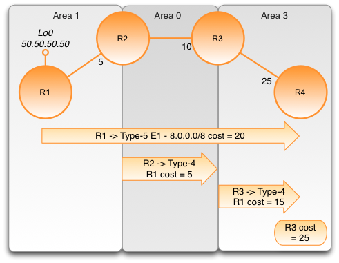
For example in above the total cost is 35 but if we had multiple hops in between each of those routers it would be calculated/propagated as follows:

R1 would advertise an lsa type 5 with Type 1 metric with an initial cost of 10 

R2 would receive the type 5 pointing towards R1, it will hence create a type 4 to assist in reachability to that ASBR outside of the local area (Type 1’s aren’t flooded outside an area)

R2 would advertise both the Type 4 (The cost R2 see’s to get to R1) and the Type 5 (The cost of the initial route)

R3 can then use the type 1 received from R2 and other type 1’s in area 0 to understand how to reach R2 and what cost that would be. 

R3 would combine the above cost and that of the type 4 and the cost of the type 5 to calculate its own cost to reach that route

R3 would then advertise the cost of the route to R2 + the Type 4 advertised by R2, in another unique type 4 for the original ASBR into area 1, R3 would also pass on the original type 5.

R4 then finally adds the two costs together from the Type 4 (15) and Type 5 (20) to get the overall cost to the network

Simple – Analyse the LSDB to find all routes, for all routes add the outgoing interface cost, pick the route with the lowest cost

Rules of route selection

Internal choice (within an area) – 

1. Finds entries based on the stub entries in the type one LSA’s
2. Runs spf to find the best route 
3. Calculate the ospf interface costs using the outgoing interface from the SPF result
4. Pick the path with the lowest cost
5. If metrics tie then equal cost load balance.

External choice (external to an area) –

1. Use type 3 information to find Subnets
2. Find the SPF to the ABR advertising X subnet with the lowest metric
3. Add the outgoing interface cost
4. If there are ties equal cost load balance.

inter/intra selection on ABR

• If more than one ABR connects to the same two or more areas, A route via the originating area will be chosen. This means traffic should prefer staying within an area than hopping through an area. 
• If a type 3 has been learnt from a non backbone source, it will be ignored when calculating its own routes (For example a dual ABR connection between area 0 and 1)

Redistributed route calculation

Internal to area

1. find the ASBR advertising the most pref’d type 5 for the subnet.
2. find the shortest path to each ASBR using the LSDB
3. Use interface costs to calculate a cost to the ASBR.
4. best cost wins. If even load balance

External to area

Instead of trying to find the best route to the ASBR directly we use the RID in the type 5 to search Type 4’s which are created by local ABR’s to advertise their reachability to the ASBR’s

So find the best Type4 to the ASBR/s needed, add costs to internal Area cost’s and find the best path.

Bandwidth/metrics

Reference bandwidth :

Interface cost = Ref bandwidth/bandwidth

Default ref is 100Mb Usually configured in kbp/s x1000

Best path is chosen with the lowest sum of the cost’s on a path.

Reference bandwidth should be configured as the largest interface in your network.
This will mean that the largest interface will have a cost of 1 while the other interfaces will have relatively higher costs based on their bandwidth.

Setting interface bandwidth

Anything defined on a physical interface will cascade down to the logical interfaces

Interface bandwidth only affects the ospf cost not the amount of traffic an interface can handle.
Isn’t the best method of Altering traffic patterns

OSPF cost manual
Interfaces can have an ospf cost assigned to them however this yet again is very laborious however it does only impact the ospf process and no other routing protocol that might be using the interface.

6 – Troubleshooting

No neighbor detected

• Check physical and link layer connectivity (show interfaces [interface])
• Check mismatched ip subnet, area number, area type, authentication, hello/dead timers and network type.
• Ensure the Link type is correct, different vendors have different defaults (point to point/multi access)

Stuck in ExStart

• Check MTU settings

Stuck in 2-way

• Normal for DR-other adjacency.

You can set ospf traceoptions to log debug information and can be viewed using show log [file name]

You can then define the level of logging by using flag options such as flag error detail

The show ospf statistics will also show you the number of receive errors the device has had since the statistics have been cleared.

Dupe RID’s

If there are dupe RID’s in the network every router will only acknowledge the first router with the Dupe RID. As the RID will already be listed in the Neighbours list.
If the routers are in different areas there is a chance devices not connected to both of them will detect them both, however this will result in a wildly changing LSDB and will cause huge amounts of messages across the network.

Mismatch MTU

If the MTU in the IP header is mismatched against the remote side, an adjacency might start as the hello messages don’t require that confirmation, however when transferring the DBD packets information will be lost due to the mismatch in sizes.

Junos TShoot notes

The Metric value in the routing table is the dynamic metric for the route shown.

When using show ospf route, you can show different types of routes. For example ASBR routes or ABR routes

When showing the ospf database it will be broken down per area. 

The sequence numbers in the DB are used to determine if lsa’s are new or not, they start with a value of 0x80000001

You can view an show ospf log to see the recent events for each type of calculation. Allows you to see if you have a stable network or not.

You can show ospf statistics to see how many of each type of packets have been sent/received by the router.

7 – Misc notes

OSPF uses 3 databases, Adjacency database, Link state database and forwarding database. 

There are different types of routers.

ABR – Area border router – At the border of a network.

Backbone – Routers in the backbone area. 

ASBR – Autonomous system border router. border between the ospf AS and an external AS

Can authenticate updates either with plain test or MD5 authentication. 

Need a key id for authentication. looks at youngest key. 

Can set authentication on an area basis or an interface basis. 

RID selection

RID’s are usually chosen based on Global configred ID but if not there then it depends on the vendor

Juniper
IP of first int to come online, usually the loopbacks

Cisco
Highest IP on loopbacks
Highest other configured Ip address

Changing timers

If you already have a formed adjacency the session won’t go down straight away.
As the settings in the hello’s won’t match between the two devices the hello’s will not be registered by the remote device.
This will result in the dead timer slowly expiring and shutting the session down.

If these timers are different they will only get up to the attempt/init state

Junos os OSPF support

There is support for MD5 and IPSec authentication of ospf exchanges.

Summarization

ABR’s send summary LSA to describe routes to other areas, You can explicitly configure a device to send out summary messages for a certain prefix.

You can configure a prefix-export-limit under an ospf process to limit the number of external prefixes exported into the network. 

Graceful restart can be enabled, this allows the routing engine to reboot without ospf adjacencies being dropped. 

This means the router rebooting will send out lsa type 9 messages, these indicate that the device is rebooting and to not end the adjacency for x number of minutes/seconds while it reboots.
See https://tinyurl.com/jgkv35p

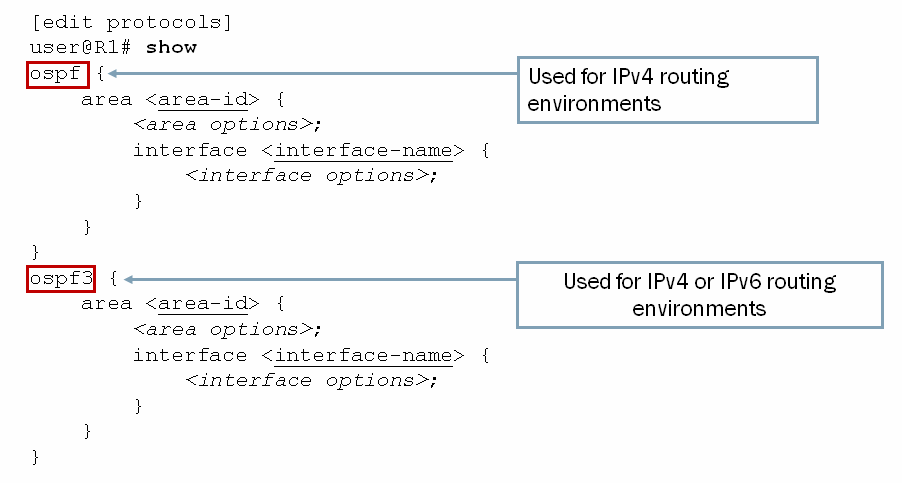
Configuration

Ospf v2 and v3 follow the same hierarchie, 

Define an area, under that the options including the interfaces in that area, and under each interface the interface options.

The Router-id can be statically configured but this is done globally under routing-options with router-id [address] 

If you have a Lo interface with a /24 address set when including that within the ospf process you will advertise both the /32 address and the /24 prefix.

If you wish to advertise a connected network but don’t wish to form any adjacencies on that network you would use the passive command under the interface options.

In the neighbour table you will see one neighbour record for each link no matter if they are all for the same remote host.

Note: when checking routing tables you will see for example [ospf/150] this will be the routing protocol and then the route preference. (Junos version of AD)

See the following for default prefixes https://www.juniper.net/documentation/en_US/junos/topics/reference/general/routing-protocols-default-route-preference-values.html